The Detection Engineering Baseline: Hypothesis and Structure (Part 1)
A practical guide to using statistical methods for empirically modeling normal in your environment

Introduction
Detection engineering has common pitfalls that show up even on experienced teams. Rules get written based on past experiences and untested assumptions, thresholds get set with limited data, and teams can end up either drowning in false positives or, worse, missing real attacks entirely. A common underlying pattern is that teams start with a detection idea, draft a rule, then rely on backtesting and threshold tuning to make it livable. Without an explicit baseline for normal behavior, that tuning tends to be reactive and fragile.
Detection baselining is the principle of using statistics, and analytical rigor to empirically model normal behavior in your environment. It’s the difference between saying “this seems like a lot of login failures” and knowing “this user is 3.5 standard deviations above their median failure rate.” It transforms detection engineering from an art into a science.
A well-executed baseline provides:
Backtesting of rule logic: Validate your detection against historical data before deploying
Codified thought process: Document why you chose specific thresholds and methods
Historical context: Capture what your environment looked like when the baseline was created
Reproducible process: Enable re-running when tuning or validating detection logic
Foundation for the ADS: Feed directly into your Alerting Detection Strategy documentation
Cross-team collaboration fuel: Surface insecure patterns and workflows with data-backed evidence
Threat hunting runway: When alert precision isn’t achievable, convert the baseline into a scheduled hunt
That last point deserves emphasis. Baselines aren’t just about building detections. They’re data-driven insights into your environment. The patterns you discover often reveal security debt, misconfigurations, and risky workflows that existed long before any attacker showed up.
Baselining uses many of the same muscles as threat hunting: exploratory analysis, hypothesis-driven questions, and deep familiarity with how your environment behaves. In this post, we’ll treat baselining as a repeatable workflow that produces both detection thresholds and environment insights you can operationalize over time.
This post walks through a complete baselining methodology using a practical example: analyzing CloudTrail API call patterns to detect unusual user activity. We’ll use synthetic CloudTrail data so you can see exactly how the statistical methods surface real threats.
The complete code, synthetic data, and notebook for this walkthrough are available at github.com/Btlyons1/Detection-Engineering-Baseline. You can follow along or use it as a template for your own baselines.
The README and Hypothesis
Every baseline begins with documentation. This isn’t bureaucracy. It’s the foundation that ensures your analysis answers the right questions and provides context for anyone who reviews your work later.
In practice, I’ve found notebooks (Juypter/Marimo/Databricks) to be the most useful and impactful medium for baselining. They let you interleave narrative, code, outputs, and decisions in one place, which makes the work easier to review and easier to operationalize. That said, nothing about baselining requires a notebook. The same principles apply if you prefer to run this as a script, a scheduled job, or a pipeline in your data platform. The important part is that the method is repeatable and the decisions are documented.
What to document
Your baseline should open with a clear statement of what you’re trying to detect, the background context (why this data source matters and what “normal” tends to look like), your hypothesis (a specific, testable claim), and validation criteria (how you’ll know if the baseline is useful). It should also capture scope: the time range, entities covered, and any known exclusions, caveats, including what you’re measuring and at what aggregation (for example, per user-day volume versus per user-hour rates).
Our example: unusual API call volume
For this walkthrough, we’re building a baseline to detect unusual per-user, per-day API call volume in CloudTrail data. Here’s our hypothesis:
Hypothesis: We can establish statistical baselines for per-user, per-day API call volume that distinguish normal operational patterns from anomalous behavior, enabling detection of unusual activity with acceptable false positive rates.
Validation criteria:
Baseline captures 95%+ of normal activity within defined thresholds
Known anomalies (injected test cases) are detected
False positive rate on historical data is < 5%
The hypothesis isn’t “detect bad stuff.” It’s a testable claim about whether your data can actually support the detection you want to build, and it forces you to define success in measurable terms. A clear hypothesis matters because baseline work expands quickly. As you dig in, you will surface edge cases and “interesting” patterns that can pull you off course. As the saying goes, if you torture the data long enough, it will confess to anything. The hypothesis and validation criteria are how you avoid overfitting your conclusions to whatever you happen to find. We’ll validate this as we work through the analysis.
Data Scope:
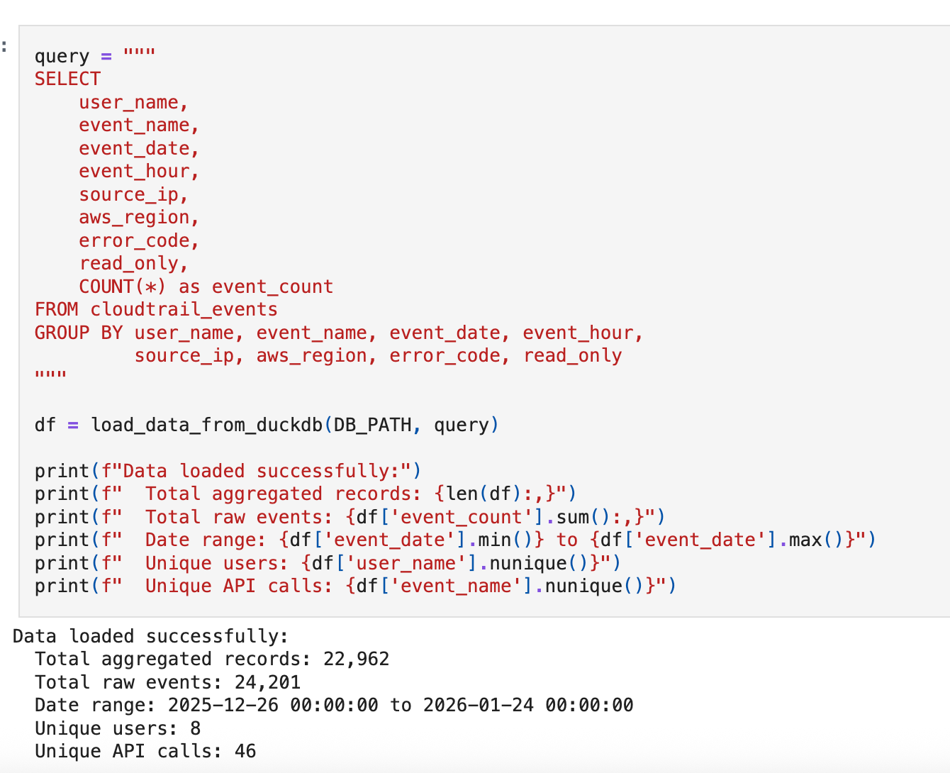
We’re working with 30 days of synthetic CloudTrail data containing 24,201 events across 8 users and 46 unique API calls.
The data includes three injected anomalies we expect our baseline to surface:
Off-hours credential creation (CreateAccessKey at 3 AM)
Bulk S3 data access (500 GetObject calls in one session)
Unknown external user making AssumeRole attempts
Environment Setup and Importing Standards
Notebooks are a great medium for baselining because they let you combine narrative, code, and outputs in one place. They also have sharp edges: cell execution order can change results, hidden state can creep in, and analysis code tends to get copy-pasted as baselines evolve.
Execution order is fragile. Running cells out of sequence can silently change state and produce results you can’t reproduce later.
Testing is awkward. It’s harder to unit test notebook cells than a Python module.
Refactoring is harder than it should be. A notebook encourages “just one more cell,” which can turn into tangled logic and duplicated code.
Consistency drifts. If every baseline re-implements statistics slightly differently, you lose comparability across baselines.
Baseline rule of thumb: if it’s reusable or testable, it belongs in a module; if it’s interpretive or explanatory, it belongs in the notebook.
That’s why I like to standardize baselining around a small set of shared helpers and a consistent baseline layout. The notebook stays focused on analysis and decisions. The helper module holds the reusable building blocks we want to keep consistent across baselines and easy to unit test.
Where baselines live
Where you store baselines is highly dependent on your setup. In some programs, it’s practical to keep baselines alongside detections and their README so everything lives in one place and review is straightforward. In others, baselines live in a separate analytics repo or directly in a data platform workspace.
The important thing is not the exact folder structure. It’s that each baseline has:
a stable identifier (detection ID)
documented scope and assumptions
versioned methodology
outputs you can reference later
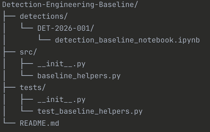
Repo structure
Project Organization:
This repo uses one folder per baseline/detection ID, plus a shared helper module. It’s designed to make baselines easy to review and keep statistical methods consistent across detections.
Outputs in practice
Outputs are environment-specific. In a real program, baseline artifacts often get written to systems that support automation and review at scale. This could be a table in Snowflake or Databricks, cloud object storage, or whatever fits your infrastructure.
The kinds of objects worth persisting include:
Thresholds and parameters (median, MAD, cutoffs)
Distribution summaries (percentiles, histograms)
Drift metrics (comparison to prior baselines)
Validation results (firing rates, entity spread)
Notebook exports (HTML or ipynb for review)
Where these land matters less than ensuring they are queryable and versioned. The repo can still capture the source of truth for methodology and documentation, while the data products land where your detection pipeline can consume them.
Helper module responsibilities
The shared helper module is intentionally boring. It centralizes logic you should not rewrite in every notebook:
data loading from common backends
robust statistics (median, MAD, modified z-score)
outlier detection utilities
frequency and concentration analysis
baseline persistence hooks (write to tables or object storage)
def calculate_modified_zscore(
    data: Union[pd.Series, np.ndarray],
    consistency_constant: float = 0.6745
) -> np.ndarray:
    """
    Calculate Modified Z-Score using MAD.

    The modified z-score is robust to outliers and preferred for security data:

    Modified Z-Score = 0.6745 * (x_i - median) / MAD

    The constant 0.6745 makes MAD consistent with standard deviation for
    normally distributed data.

    Parameters
    ----------
    data : array-like
        Numeric data to analyze
    consistency_constant : float
        Constant for consistency with normal distribution (default: 0.6745)

    Returns
    -------
    np.ndarray
        Modified z-scores for each data point

    Reference
    ---------
    Iglewicz, B. and Hoaglin, D.C. (1993). How to Detect and Handle Outliers
    """
    data = np.asarray(data)
    median = np.median(data)
    mad = calculate_mad(data)

    # Handle case where MAD is 0 (all values are identical)
    if mad == 0:
        return np.zeros_like(data, dtype=float)

    return consistency_constant * (data - median) / mad
With the hypothesis defined, the dataset scoped, and the helper module in place, we have everything we need to start analyzing.
In Part 2, we will work through the analytical core of baselining: frequency analysis to understand concentration and rarity, robust statistics to score anomalies without being distorted by outliers, and contextual grouping to capture what “normal” actually means for different entities in your environment. By the end, we will have surfaced our injected anomalies and built a foundation for detection thresholds.
Part 1 Recap
This post established the foundation for evidence-based detection engineering:
A clear hypothesis. We are testing whether per-user, per-day API call volume in CloudTrail can reliably distinguish normal activity from anomalies. We defined validation criteria so we will know if the baseline succeeds.
Documented scope. We know the time window, the entities covered, the metric we are measuring, and the injected anomalies we expect to surface.
A repeatable structure. Baselines live in a consistent folder layout with a shared helper module. The notebook handles interpretation and decisions. The module handles reusable statistical logic.
A mindset shift. Baselining is not just about picking thresholds. It is about empirically modeling normal behavior so that detection decisions are grounded in data, not intuition.
None of this required writing a single detection rule. That is intentional. The upfront investment in hypothesis, documentation, and structure pays off when you need to validate, tune, or explain your work later.
Next, we start analyzing. Part 2 covers frequency analysis, robust statistics, and contextual grouping, the technical core that turns raw telemetry into actionable baselines.