The Detection Engineering Baseline: Statistical Methods (Part 2)
A practical guide to using statistical methods for empirically modeling normal in your environment

Building the Statistical Backbone
In Part 1, we established the core premise: effective detection engineering starts with understanding what's normal before writing rules about what's suspicious. We walked through hypothesis formation, environment setup, and importing detection standards. Now we move into analysis.
This post covers the statistical backbone of baselining: frequency analysis to understand concentration and rarity, robust statistical methods that don’t collapse under the weight of outliers, and grouping strategies that let you apply those methods where they matter. By the end, you’ll have a repeatable framework for turning raw telemetry into defensible thresholds and a clearer picture of what “anomalous” actually means in your environment.
Frequency Analysis
Frequency analysis answers a few foundational questions up front: what happens most often, what's rare, and whether activity is concentrated among a few high-volume actors. Those answers shape everything downstream: whether a global threshold is plausible, which entities need their own baselines, and where rarity alone is worth a closer look.
Understanding the Long Tail
Security telemetry almost always has long-tail behavior. A small number of users, APIs, hosts, or service principals account for a disproportionate share of events. If you don’t account for that concentration, detections based on raw counts tend to either over-alert on high-volume actors or completely miss low-and-slow anomalies in the tail.
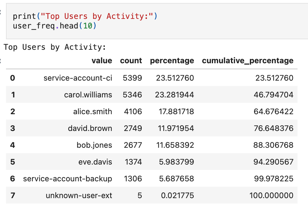
This tells us that 4 users generate ~90% of CloudTrail volume. That’s a strong signal that a single global “events per day” threshold will be fragile. Service accounts and CI principals often generate high volumes by design. In contrast, human users are typically lower volume and more variable. This is exactly where per-entity baselines or cohort-based grouping become necessary.
Cohorting means grouping similar entities together (service accounts with service accounts, developers with developers) so you can apply shared baselines to entities that behave similarly rather than treating every identity as unique.
Frequency analysis is also where you pressure-test the metric you chose in the hypothesis. Here, we’re baselining per-user, per-day volume. The distribution and concentration metrics tell us whether that unit is stable enough to model, or whether we need to refine the approach. Common refinements in CloudTrail include moving to per-hour rates for bursty activity, or baselining changes in a user’s API call set when volume alone isn’t discriminative.
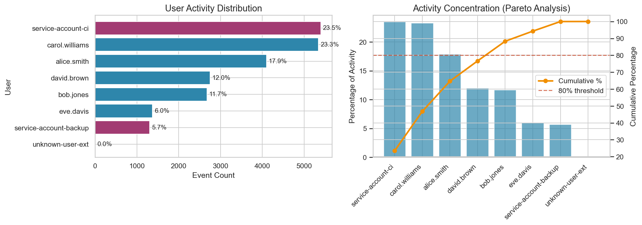
Pareto analysis
Pareto analysis is named after the observation that a small portion of causes often accounts for most of the effect (the “80/20 rule”). The chart shows individual counts alongside cumulative percentage. In this dataset, 5 users cross the 80% line. These are your “head” entities, candidates for individual baselines because their behavior is distinct and high-impact. Everyone below is the “tail,” often better served by cohort-based thresholds or shared rules.
Your data may not split this cleanly. Concentration could be more extreme (a single service account generating 60% of volume) or flatter (no clear break point). The goal isn’t to hit 80/20 exactly; it’s to identify where concentration exists and use that to decide how to group your baselines.
Identifying Rare Events
Rare API calls are often worth attention because they can map to privilege changes, unusual administrative actions, or workflows that only occur during incident response and break-glass scenarios. They are not automatically malicious, but rarity is a useful triage signal in a baseline because it tells you what’s uncommon in your environment.
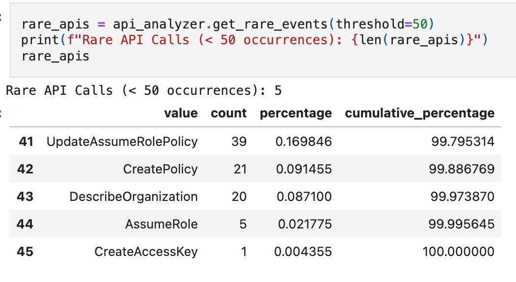
That single CreateAccessKey call is one of our injected anomalies, and it stands out immediately in frequency analysis.
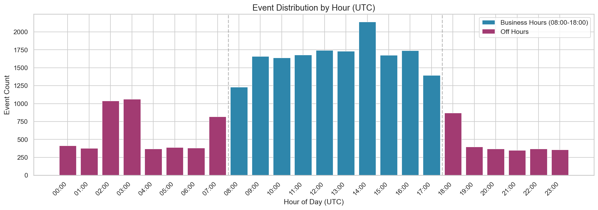
Temporal Patterns
This shows a clear “business hours” pattern in UTC. In a real environment, you’d translate this into expected working hours for your org and known scheduled jobs. Off-hours activity is often a useful dimension to carry forward, especially when combined with user type (human vs service account), source IP, and API type. We’ll use this off-hours ratio as a context dimension later in this post.
Statistical Distribution Analysis
Frequency analysis told us what happens and how often. But knowing that one user generates 500 events while another generates 50 doesn't tell us whether either is abnormal. For that, we need to quantify deviation, and that means choosing statistical methods that won't break the moment an outlier shows up.
At this point we know the data isn’t evenly distributed. A handful of identities generate most of the volume, and rare events show up as sharp spikes. That’s exactly the kind of dataset where naive thresholds fail, so we need robust statistics.
This is where many detection efforts go sideways. It’s tempting to reach for familiar formulas, but security telemetry rarely behaves like textbook data. The statistical methods you choose determine whether your thresholds are defensible or arbitrary.
Why Mean and Standard Deviation Are Brittle in Security Data
Security data is usually right-skewed with heavy tails. Most observations cluster at low values while a small number of extreme days pull the distribution to the right. Those extremes might be benign bursts, misconfigurations, or attacks, but either way they distort mean and standard deviation in ways that matter for detection thresholds.
Let’s aggregate our data to daily volumes per user and examine the distribution:
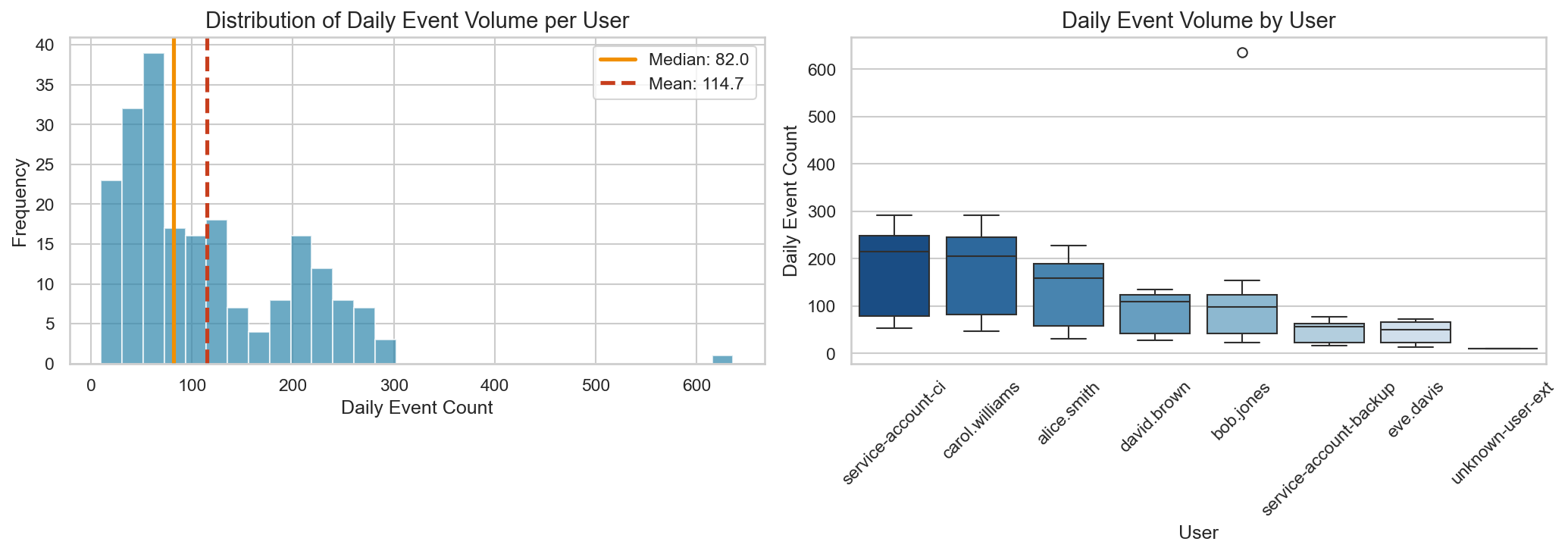
The mean (114.7) is ~40% higher than the median (82.0). In this dataset, one anomalous day with ~620 events (our injected bulk data access) contributes meaningfully to that gap. If you build thresholds directly from mean and standard deviation, a small number of extremes can heavily influence where "normal" ends and "anomalous" begins.
The boxplots on the right hint at why global thresholds fail: carol.williams and service-account-ci have wide daily variance, while eve.davis is tightly clustered. A threshold that works for one will misfire on the others.
Robust Statistics: Median and MAD
Robust statistics are designed to remain stable even when the dataset contains outliers.
Median: The middle value when sorted. Resistant to extreme values.
MAD (Median Absolute Deviation): A robust measure of spread:
For each value, calculate its distance from the median, then take the median of those distances:
Daily counts: [50, 60, 82, 90, 620]
Median: 82
Absolute deviations: [32, 22, 0, 8, 538]
MAD: 22 (the median of the deviations)
Notice how the 620 outlier doesn’t drag MAD up the way it would drag up standard deviation.
The Modified Z-Score
The modified z-score replaces mean/std with median/MAD1:
You might notice the constant 0.6745 in the formula. This isn’t a magic number; it’s a scaling factor.
In a perfectly normal (Gaussian) distribution, the Median Absolute Deviation (MAD) is approximately 0.6745 times the standard deviation. Mathematically, this value comes from the inverse of the 75th percentile of the standard normal distribution:
Why does this matter?
The constant 0.6745 scales the MAD so that it estimates a standard deviation. This lets you interpret modified z-scores the same way you would standard z-scores: in a normal distribution, about 99.7% of data falls within 3 standard deviations of the mean. A modified z-score of 3.52 represents a similar level of rarity, but calculated using robust statistics that won't be distorted by outliers.
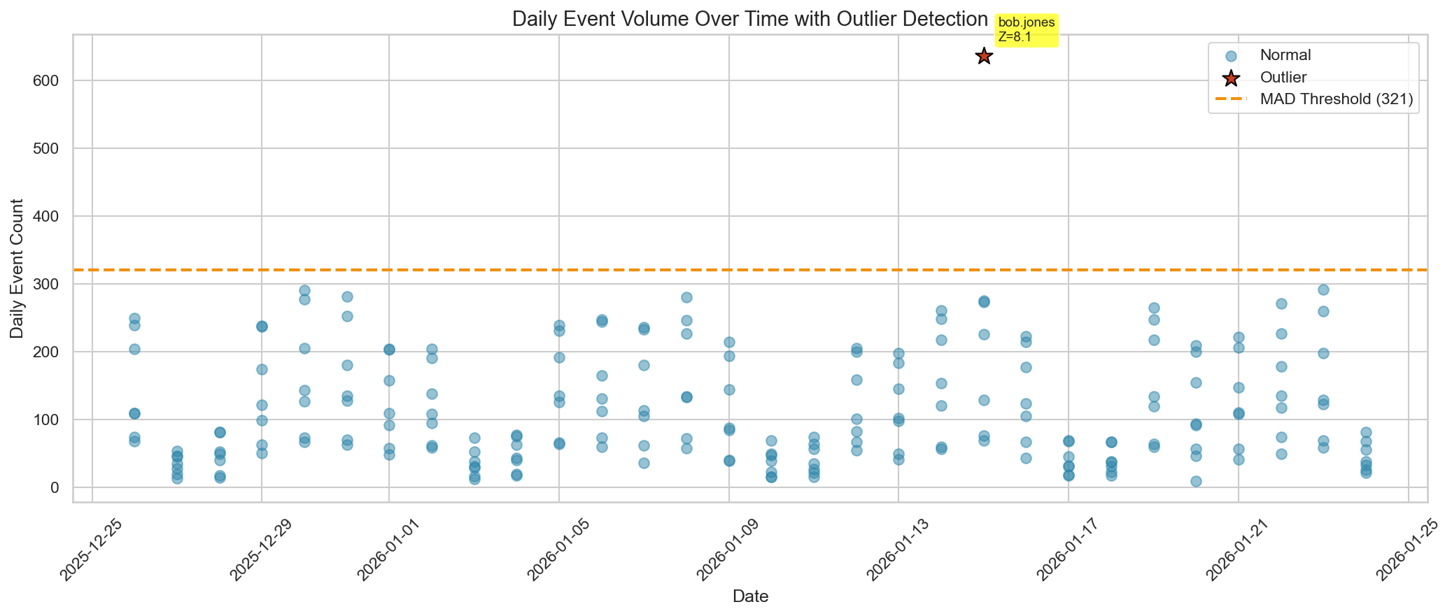
Our baseline surfaced exactly one statistical outlier: the injected bulk data access. More importantly, it did so using a method that remains stable even when the dataset contains extremes.
Threshold Comparison
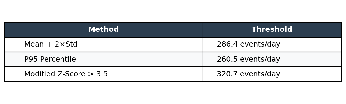
The Modified Z-Score threshold is computed as:
threshold = median + (3.5 × MAD / 0.6745)
threshold = 82.0 + (3.5 × 46.0 / 0.6745)
threshold = 320.7
These thresholds land in the same general range, but they behave differently and answer different questions.
Percentiles are simple: P95 means 5% of observations exceed this value. But percentiles don’t tell you how abnormal something is. A value at P96 and a value at P99.9 both just “exceed P95.” You also have to pick the percentile arbitrarily. Why P95 and not P99?
Mean + standard deviation gives you a measure of distance from center, but it’s sensitive to the same outliers you’re trying to detect. One bad day can shift your threshold significantly.
You could argue: just set the threshold once and don’t recompute. But static thresholds degrade over time. Your environment changes, new service accounts spin up, workloads shift. A threshold that made sense six months ago might now fire constantly (too many false positives) or miss everything (too permissive). You need a method that can be recomputed safely as new data arrives.
Modified z-score gives you that stability. Because it's built on median and MAD, adding new outliers to your dataset doesn't drag the threshold around. You can recompute weekly or monthly without worrying that one bad week will ruin your baseline. And you get an interpretable score for every observation. That score becomes a building block: you can set tiered alert severities, track whether an entity's behavior is drifting over time, or combine it with other signals like timing and API rarity. A binary threshold tells you "anomaly or not." A score tells you how anomalous, grounded in quantifiable evidence from your own environment.
Data Grouping and Aggregation
The previous section gave us robust scoring methods. Now we decide where to apply them. In long-tail datasets, grouping choices often matter more than the exact cutoff because “normal” is not global. It’s contextual. A CI service account, an on-call SRE, and a developer all generate different shapes of activity that can be legitimate.
Start with Per-Entity Baselines
Because our hypothesis is about per-user, per-day volume, the first grouping decision is straightforward: baseline volume per user, not globally. This is the simplest way to avoid penalizing high-volume accounts while still detecting truly unusual spikes.
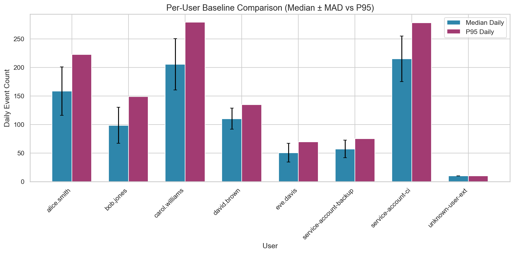
Two things stand out immediately:
The baselines are meaningfully different across users. That’s expected, and it’s exactly why a global threshold is brittle.
unknown-user-exthas only one active day. Low volume isn’t automatically safe. A brand-new identity with any sensitive behavior can be high-risk even if the count is small. For new entities without enough history, you may need to fall back to cohort baselines or apply stricter scrutiny by default.
Add Context Dimensions That Change How You Interpret Volume
Volume alone often isn’t enough. The same daily count can mean different things depending on when it happened, where it came from, and what it targeted. Baselining gets more useful when you add a small number of high-leverage dimensions.
Temporal Patterns: Off-Hours Ratios
Many environments have clear time-of-day patterns. Instead of treating “off-hours” as inherently suspicious, the baseline should capture whether off-hours activity is normal for that identity type.
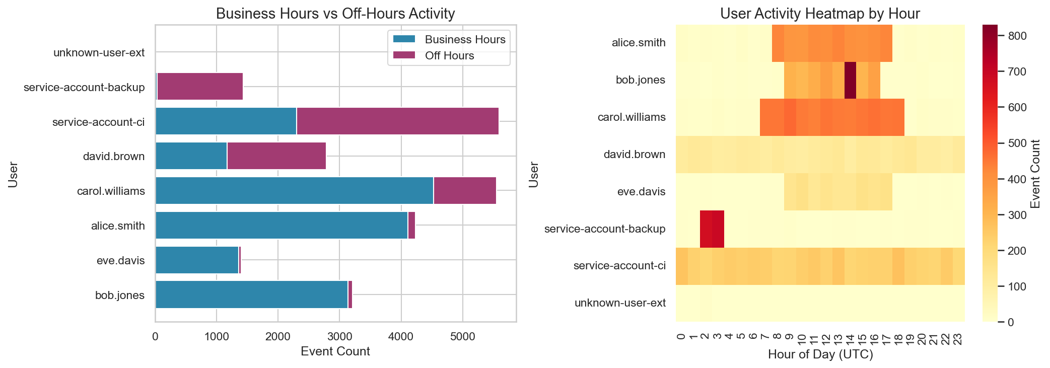
This is a good example of why context matters:
service-account-backupbeing ~98% off-hours is expected if backups run overnight.A typical developer being ~3% off-hours is also expected.
unknown-user-extbeing 100% off-hours is a strong signal when combined with other indicators (identity maturity, source IP, API types).
This doesn’t mean “off-hours equals bad.” It means off-hours is a useful multiplier when it deviates from a baseline for that entity or cohort.
Source IP Context: Internal vs External
Source IP is often one of the simplest and often valuable groupings in CloudTrail baselining. The goal is not to perfectly classify all traffic, but to quickly surface identities whose access patterns don’t match expectations.
Other fields can serve the same purpose depending on your environment: the first four characters of an access key ID indicate the key type (AKIA for long-term, ASIA for temporary, etc), user agent strings can flag unexpected tooling (especially if your org standardizes on internal tooling, specific CLIs or SDKs), and resource ARNs can reveal access to sensitive assets. The principle is the same: find fields that distinguish expected from unexpected access patterns in your environment.
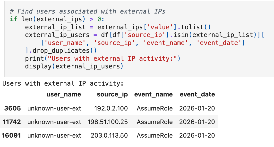
In this dataset, the signal is obvious: three external IPs3, one unknown user, all calling AssumeRole on the same day. Real environments are messier. Legitimate external access can come from VPNs, contractors, mobile users, cloud services, partner integrations, and more. The baseline helps you know which external access is expected so you can focus on what isn't.
When you surface a combination like this: a previously unseen identity, external-only source IPs, and sensitive APIs like AssumeRole, you have a strongly prioritized lead grounded in baseline context, not intuition.
Putting It Together
We started with a hypothesis about unusual CloudTrail volume per user. Frequency analysis showed us where activity concentrates and which APIs are rare. Robust statistics gave us a scoring method that doesn’t break when outliers appear. Grouping and context dimensions told us where to apply that scoring and what additional signals matter.
Now we can build detections with teeth. For our example, a detection could fire when a user’s daily volume exceeds a modified z-score of 3.5 against their own baseline. That alone caught the injected bulk access anomaly. But we can do more. We can create tiered severities: z-score above 3.5 is medium, above 5.0 with off-hours activity is critical. We can add conditions: only alert if the source IP is external or if the API is in our rare set. We can build separate detections for different risk profiles: one for service accounts, another for human users, another for new identities with no baseline history.
The same analysis also tells us how the environment actually works. We know which users drive volume, what time of day activity peaks, which APIs are routine versus exceptional. That understanding doesn’t just power detections. It makes investigations faster because you already know what normal looks like. It surfaces questions worth asking, like why a single service account touches 15 different AWS services or why a developer role has KMS decrypt permissions it never uses.
And the data can drive broader security improvements beyond detection. Baseline findings become evidence for implementing security controls like Service Control Policies that restrict sensitive APIs to specific roles. They inform paved paths for secure development by showing what access patterns legitimate workflows actually need. They give you leverage in conversations with platform teams because you’re not arguing from intuition. You’re showing them what their environment is doing.
This is what evidence-based detection engineering looks like. The statistics aren’t decoration. They’re the foundation that makes everything else defensible.
What’s Next
In Part 3, we'll validate this baseline against known anomalies, measure expected firing rates, and decide whether the output becomes a detection, a scheduled hunt, or environmental insight. We'll look at how baseline findings surface security debt and become leverage for cross-team conversations that drive real change. And we'll cover how to persist your work and where AI and LLMs can reduce the toil without sacrificing rigor.
Note on Asymmetry: While Modified Z-Score is robust to outliers, it mathematically assumes the underlying data is roughly symmetric around the median. For strictly positive, heavy-tailed metrics (like “Bytes Transferred” or “Session Duration”), the distribution remains asymmetric even after cohorting. In these specific cases, applying Modified Z-Score to raw data can still yield excessive false positives on the “high side.” A common refinement is to apply a log-transformation (e.g., Log(x+1)) to the data before calculating the Modified Z-Score.
Why 3.5? The threshold of 3.5 comes from Iglewicz and Hoaglin's work on outlier detection. It balances sensitivity with robustness. In practice, you'll tune this based on your environment's tolerance for false positives. Start at 3.5, backtest against known-good and known-bad periods, and adjust.
These IPs (192.0.2.x, 198.51.100.x, 203.0.113.x) are RFC 5737 documentation ranges, not routable on the public internet. In this synthetic dataset they represent external access. In production, you'd see actual public IPs here.
References
Modified Z-Score and Outlier Detection
Iglewicz, B. and Hoaglin, D. (1993). How to Detect and Handle Outliers. ASQC Quality Press. PDF
MAD Scaling Factor (0.6745)
Rousseeuw, P.J. and Croux, C. (1993). “Alternatives to the Median Absolute Deviation.” Journal of the American Statistical Association, 88(424), 1273-1283. PDF
Accessible Overviews
NIST/SEMATECH e-Handbook of Statistical Methods, Section 1.3.5.17: Detection of Outliers
Statology: What is a Modified Z-Score?